How to create a calendar template in Gnumeric that can be updated dynamically by changing the year or the month. This tutorial includes a downloadable template (.gnumeric).
In this post I will guide through the steps of making an editable calendar template for Gnumeric in which you can easily change the month or year and the full calendar gets updated.
For those looking for a Gnumeric calendar template that they just want to print, simply download one of the two files below:
If you’re interested in other designs or styles check out the PDF calendars here.
As a quick review of Gnumeric, I can say that I didn’t encounter any major issues and I was able to do what I needed. It has a simple interface and it is very fast to launch, even inside an underpowered VM.
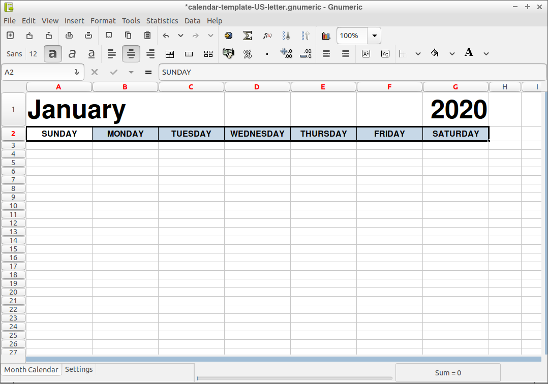
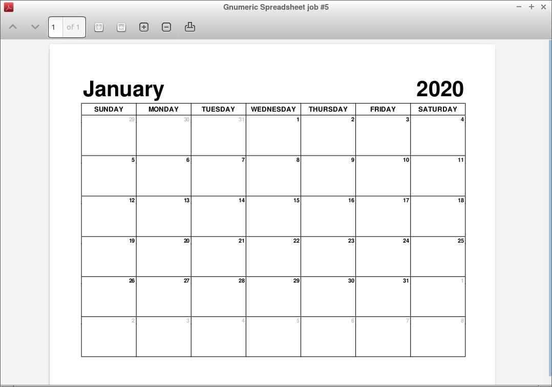
Before we get started, here is the end result, so you know what to expect:

Let’s begin by making a new spreadsheet. From the top menu choose File, then New.
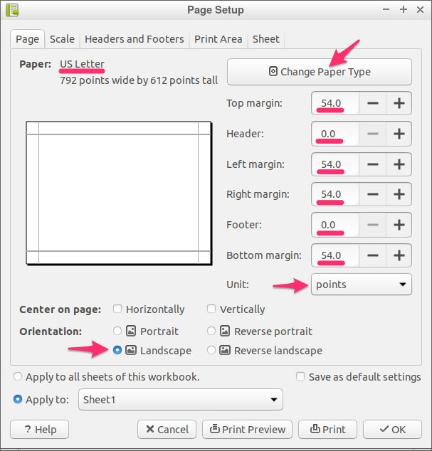
To be able to print this calendar and still get a nice result, we’ll need to update the default page settings. That can be done by going to File -> Page Setup…
If needed, click on the “Change Paper Type” button to choose “US Letter” as the paper size. From the “Unit” dropdown select “points” (you’ll see later why).
We can hide the Header and Footer by giving them a “0” value. For the margins I chose 54 points (that’s about 0.75 inches). Finally, select “Landscape” for the the “Orientation”.
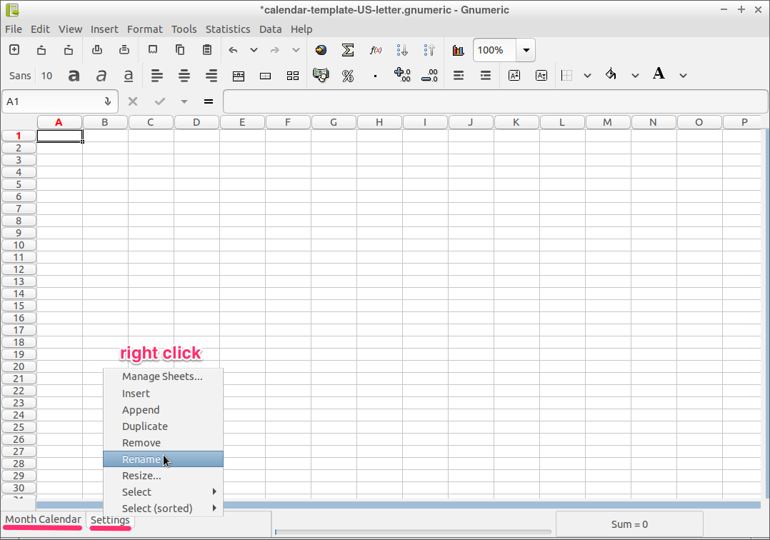
By default, Gnumeric will create three sheets in a new spreadsheet, but we only need two for this project. So delete the third sheet and rename the first two. I chose “Month Calendar” for the 1st sheet and “Settings” for the second one.
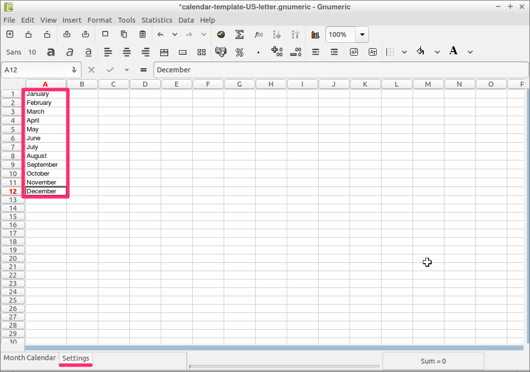
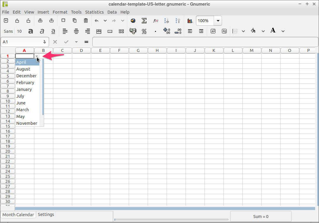
To avoid mistakes and typos we can define a list of month names in advance. We’ll use the “Settings” sheet for that. In theory, you can write the month names in any language, but in this tutorial I’ll stick with English for obvious reasons.
So switch to the “Settings” sheet and, in the first column, write the month names below each other.
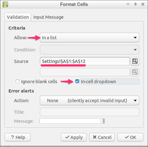
We’ll use this list of month names as the source for a drop-down. In the “Month Calendar” sheet select the first cell (A1). Then, go to Data -> Validate….
A panel called “Format Cells” should appear on the screen. Under the first tab, “Validation”, select “In a list” from the “Allow” options. Then in the “Source” field write this formula: Settings!$A$1:$A$12. This will get all the cells in the “Settings” sheet that are in column A from row 1 to row 12. Finally, tick the “In-cell dropdown” checkbox and click “OK”.
Now you should see a button with an arrow pointing down next to the first cell. If you click on that button you should see a drop-down list with all the months. Unfortunately, at least the version I have (1.12), Gnumeric automatically sorts the month names alphabetically. So the result is not ideal, but still better than having to type the month name.
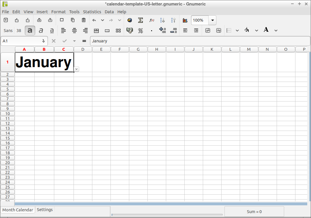
It might be a bit soon, but we’ll have to start styling things. Let’s begin by making the month larger. I chose the default font, Sans, size 38, bold. Another thing I did was to merge the first 3 cells, to have more space.
Now it’s time for some math. We need to calculate the width of a day, which in our case is the same as the width of a column. There are 7 days in a week, so we’ll use 7 columns. Because of this, we’ll have to divide the width of our page to 7. A quick glance at the page settings will give us the info we need. Go to File -> Page Setup…
Get your calculator application ready. To get the column width I take the page width from which I subtract the margins and divide the result to 7: (792-2*54)/7 = 97.71. Don’t worry if you get a long number, we only need the first two decimals(and maybe not even those).
To resize the columns select the first 7. Then from the menu choose Format -> Column -> Width… and you should get a panel where you can sort of use the result of what we calculated.
Remember at the beginning when I used points for the page width and margins instead of inches? This is why. And even points are not directly usable. We have to give the value in pixels. Luckily, this value gets translated into points, so we can approximate it.
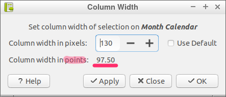
As you see in the image above 130 pixel is 97.5 points which is the closest I can get to my value, 97.71, and not go over it.
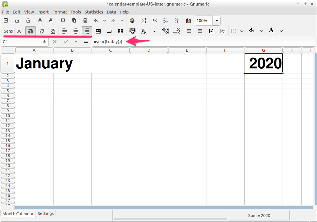
Now that we have the column width set, let’s get on with building the calendar. Following the design, we should have the year on the right, all the way at the top. So in the G1 cell, type in the year you want. To keep this template dynamic, I chose the current year given by the formula =YEAR(TODAY()).
Next, we write the days of the week in the row under the month and year. In this case, the week starts on Sunday. If you’re looking for an example with the week starting on Monday, check out the A4 calendar template.
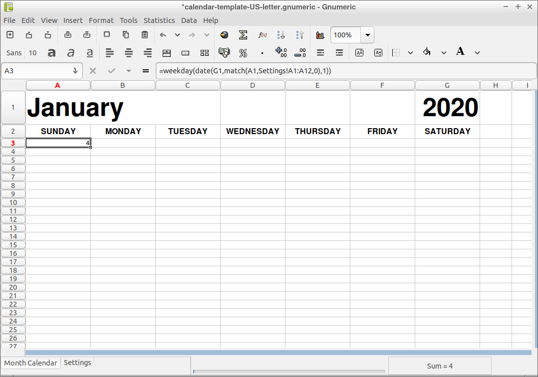
With the top section ready, we can continue with the rest. For that, we have to know what the first date in our calendar is. Unfortunately, it’s not the 1st of the current month, that would be easy, but it’s one of the last days in the previous month. The good thing, though, is that once we know that date, we just add 1(one day) to that value until we have six rows. Why 6 rows, I’ll tell you a bit later.
So how are we going to get that first date? In the A3 cell, we’ll begin by getting the first day of the month. This formula should give us exactly that =DATE(G1,MATCH(A1,Settings!A1:A12,0),1).
To untangle this formula a bit, let’s take the DATE function first which has 3 parameters: year, month and day. The year is easy, we can get it from G1. The month, however, has to be a number, but we only have “January” to work with, which Gnumeric cannot translate into a number from 1 to 12. The solution is to try and find the position of the word “January” in the month list available in the “Settings” sheet. Here’s where the MATCH function comes in handy. It needs the value you’re looking for(A1 in our case) and the cell range where to look for it(A1:A12 in Settings). The last parameter, “0” is required to only match exact values, which is what we want.

Of course, putting the first day of the month in the first cell is not correct, because most months don’t start on a Sunday. But it’s a good starting point.
Knowing the first day of the month can get us the corresponding day of the week. The function that does that is called WEEKDAY and this is the formula we need =WEEKDAY(DATE(G1,MATCH(A1,Settings!A1:A12,0),1)). The result should be a number from 1 to 7. In case it isn’t (and it’s not an error) try changing the format from “Date” to “General”.
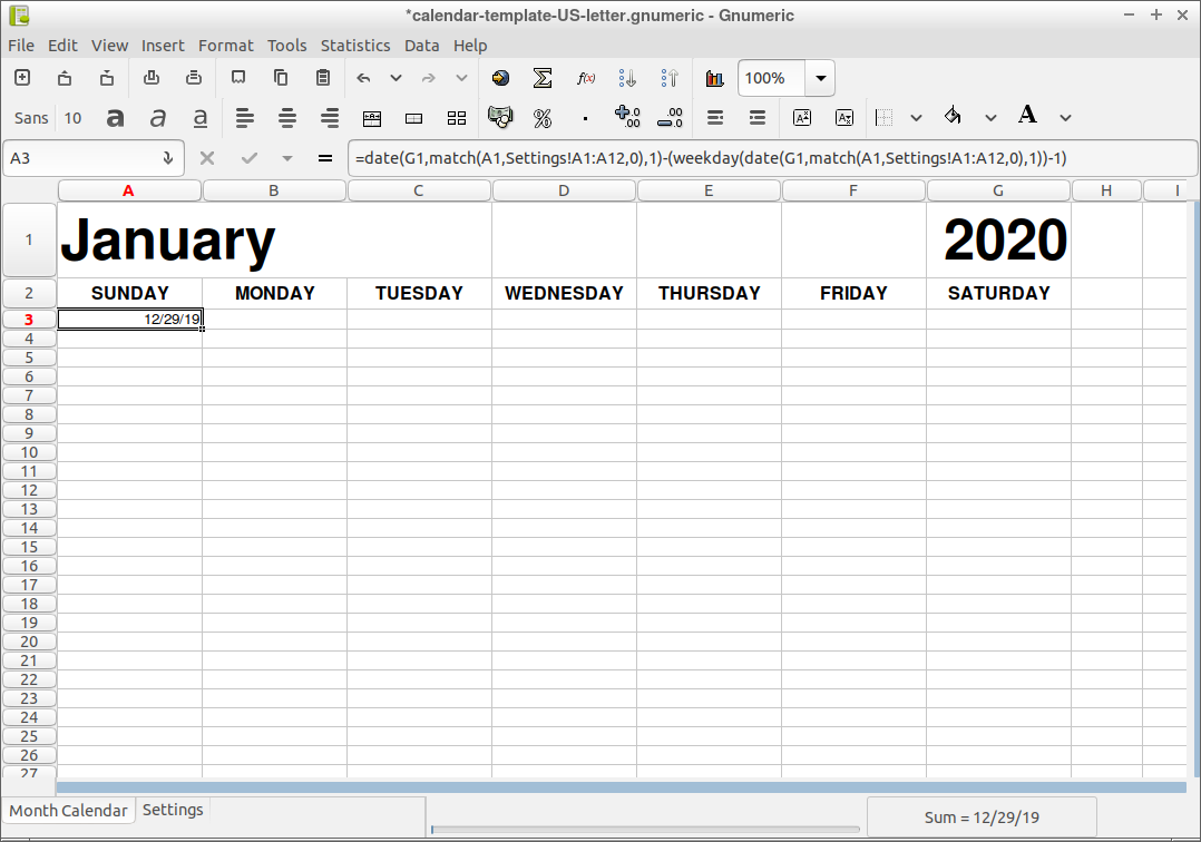
If you’re wondering why do we need the weekday, a real example might make it easier to explain. In my case, the week starts on Sunday, which makes Wednesday the 4th day of the week. That means that if the 1st of January falls on a Wednesday(the 4th day), then Sunday would have been 3 days before – on the 29th of December. So we simply need to subtract 3 days from the date which is the 1st of the month. This is the rather long formula which we need: =DATE(G1,MATCH(A1,Settings!A1:A12,0),1) - (WEEKDAY(DATE(G1,MATCH(A1,Settings!A1:A12,0),1)) - 1).
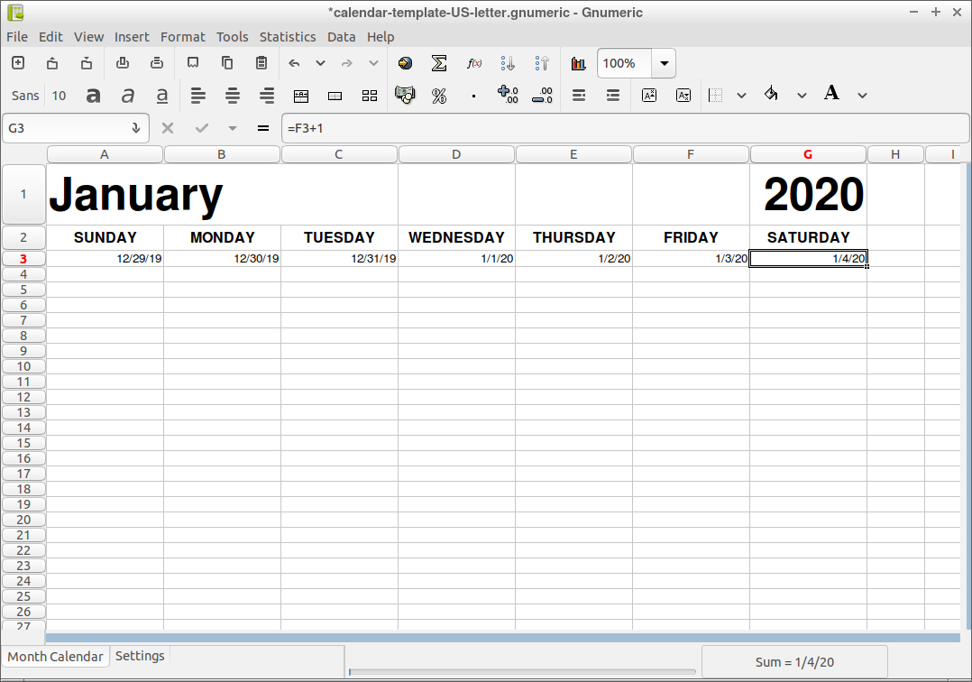
Now that we have the first date in our calendar all we need to do is add one to the previous row cell. So B3 will be =A3+1, C3 will be =B3+1 and so on until the end of the week.
We’ll keep the following row empty because, as you saw in the design, we need some space that stays editable. This means the next cell we’ll use is A5. Instead of just adding 1 day to A3, we’ll now add 7 which results in =A3+7, =B3+7 and so on till the end of the second week. Following this pattern, we need to skip the 6th, 8th, 10th and 12th row. Then we have A7 =A5+7, A13 =A11+7 and so on until our calendar is complete.
Quick Tip: copying row 5 and pasting into row 7, will save you some time from typing as Gnumeric will auto-update the values.

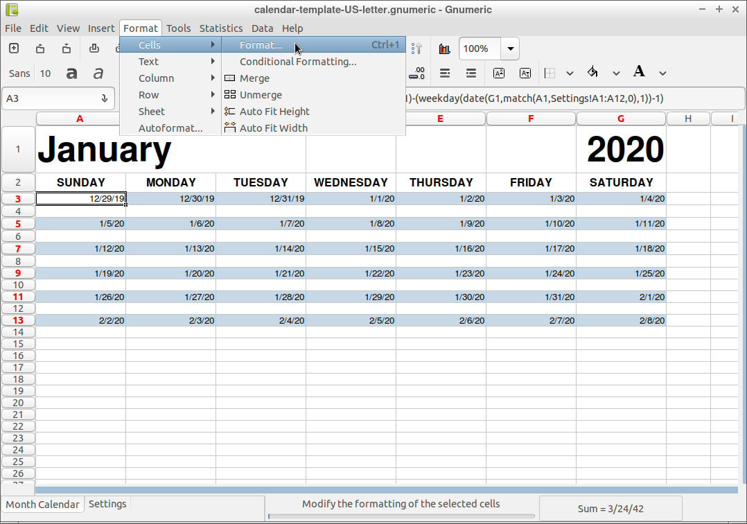
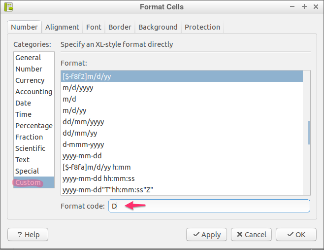
We’re making progress, but we don’t want the year and month for each day. To only show the actual day number, select all the cells containing dates(you can do it one by one or hold down the Ctrl key and click on the cells you want to select). Then from the menu bar choose Format -> Cells -> Format…
In the “Format Cells” dialog select “Custom” from the “Categories” list. Then, in the “Format code” field, type “D” and click OK.
This is up to you, but I chose to make the day text bold.
The next step involves some simple math. We need to make sure the calendar also fits vertically in the page. In the beginning we calculated the width of the columns, now we need to calculate the height of the empty rows. The empty rows or gaps are the space where we can write notes or events for a certain day.
First, lets remind ourselves how tall the page is again. Under File -> Page Setup, I can see it’s 612 point in height. From that number I also have to subtract the top margin which is 54 points and the bottom margin which is also 54 points.
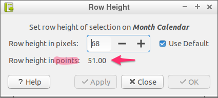
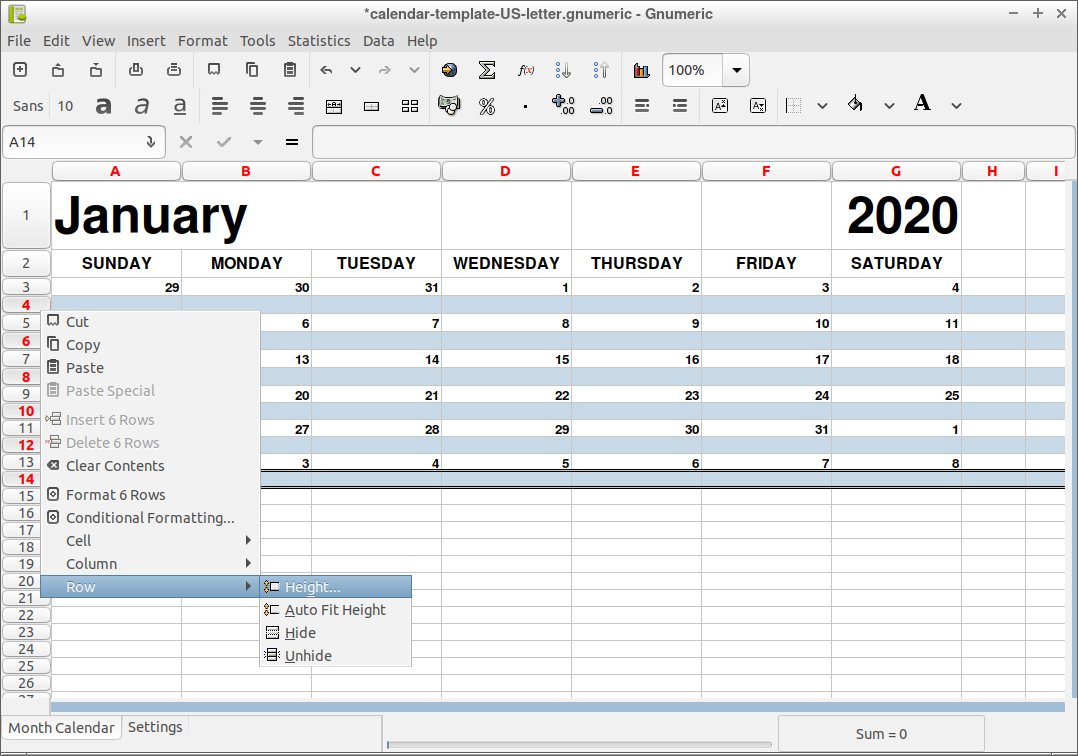
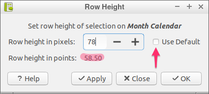
Next we need the height of all the rows with text in them. To find the height of a row right-click on it, select “Row” and then “Height…”.

Very important! Remember to write down the points value, not the pixels one.
Now we get to calculate the height for the empty rows. We have the height of page, 612, then the top and bottom margins 108 (54*2) and the height of the filled rows, 153. So 612 - 108 - 153 = 351.
All that’s left to do is divide 351 by 6(there are six weeks in our calendar). The result is 58.5 points. That’s how tall the empty rows should be, so they can nicely fit in the page.
Very important! Uncheck the “Use Default” option and remember: we are working with points not pixels.
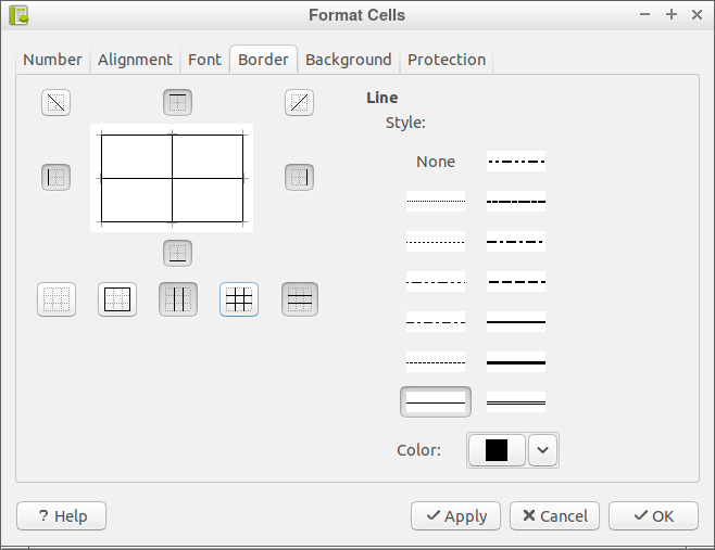
Let’s add some more styling to our calendar. I’m talking about borders. Make a selection like you see in the image below:

Then from the menu bar go to Format -> Cells -> Format…. In the “Format Cells” panel choose the “Border” tab. Here, click on the “Outline” icon/button and on the “Inside” icon/button. To confirm the changes, click OK.
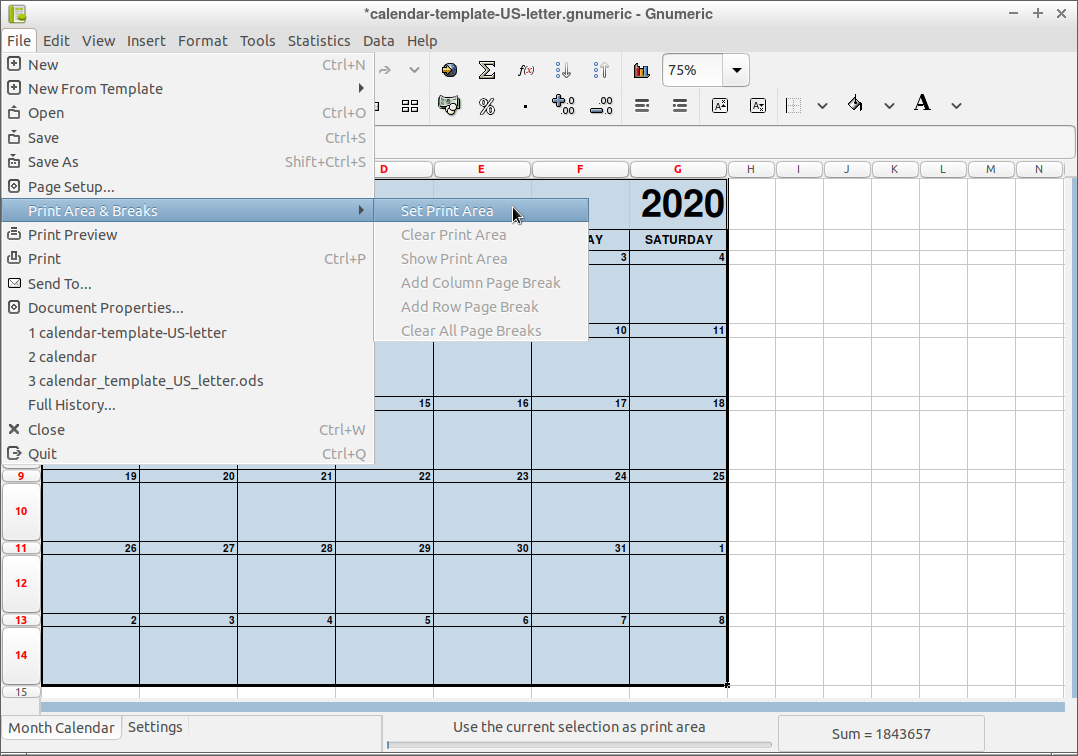
Before we preview the result, we need to define a print area. Make a selection like the one you see below and from the menu choose File -> Print Area & Breaks -> Set Print Area.
Let’s now check how “Print Preview” looks like.

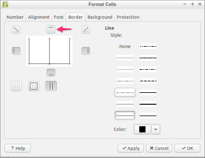
We can make it a bit nicer by “joining” the date cell with the corresponding event one. We need to only remove the top border from the event cells in order to achieve this effect.
So select the event cells then go to Format -> Cells -> Format…. Under the “Border” tab of the “Format Cells” panel simply click on the “Top” icon/button to toggle the visibility of the top border.
One final look at the end result:
For those wondering how to make the days in the previous and following month to be less visible, I can tell you it involves “Conditional Formatting”. Downloading the calendar template will give you an idea how it works. If there will be enough interest in this tutorial, I will add that part as well to this post.